Blender Rendering on a SLURM Cluster

Background

Currently I am working on a movie of our accelerator ring. The movie will be a camera flight along the ring and will consist of more than 5000 frames to realize a sequence of about 2 minutes length. The blender file is more than 800 MB of size and rendering one frame (30 samples per pixel) on my local quad-core i5 machine (I do have as well a CUDA graphics card) takes about 5 hours as I am using effects like depth of view, a couple of lights in the scene, full global illumination, etc.
Fortunately, at work we have a high performance computing cluster (see https://www.gsi.de/en/work/research/it/hpc.htm) with 550 linux machines offering a maximum of 13800 CPU cores, using SLURM as job manager to distribute the jobs among the cores.

Blender@SLURM: not Always Easy

To use the possibilities of our HPC cluster, I started programming a batch script which submits the following blender command line command to the cluster system:

blender -b <myBlenderFile>.blend -o <output path> -F PNG -s <startFrame> -e <endFrame> -a

which needs to be called via a Linux bash shell script. This command line command calls Blender in batch mode ("-b") and renders an animation set ("-a") from frame "-s" to frame "-e". The output path is specified using the "-o" command.

I started in a naive approach and ended up in frustration. Simply by putting the command above in to a shell script (including the "#!/bin/bash" command as first line) led to errors: the cluster refused to accept the script and always bailed out with an error "slurmstepd: error: Exceeded step memory limit at some point."


With some help of our local experts, I found out that this error is due to the memory-management of Blender: Where the SLURM cluster is able of assign memory per CPU-core (in my case Blender wanted 4GB in total), where Blender is not able to handle memory per core, but requires to have exclusive access to a machine's memory.


Another point is the run time of the job(s). As I said, the run time on a 4 core machine is about 5 hours; the SLURM cluster machines have Xeon processors with up to 40 cores, reducing the run time to something like 15 minutes, depending on the actual hardware. However, this adds up to a total run time for the whole movie of 5000 frames to something like 1200 hours, which is 50 days of CPU time. This means, I would like to perform as much parallel processing as possible. On the other hand, our SLURM cluster by standard does not allow more than 6 hours of run time, which means I cannot render more than 24 frames per submitted batch.

SLURM Shell Script

After some tries I ended up with the following script ("renderAnim.sh") to render the movie:

#!/bin/bash
# Task name:
#SBATCH -J <default job name>
#SBATCH --mail-user=<email address for notification>
#SBATCH --mail-type=FAIL
#SBATCH --time=4:00:00
#SBATCH --exclusive
# Working Directory on shared storage
#SBATCH -D <path to working directory>
# Standard and error output
###SBATCH -o %j_%N.out.log
#SBATCH -e %j_%N.err.log
# Application code
if [ $1 -eq $2 ]
then
    PATH=<if you need a local blender installation put PATH here>
    blender -b <myBlendFile>.blend -o ./output/ -F PNG -s $1 -e $2 -a
else
    if [ $2 -lt 5000 ]
    then
        OLD_END=$2
        NEXT_START=$((OLD_END+1))
        NEXT_END=$((OLD_END+10))
        sbatch --job-name=${NEXT_START}_${NEXT_END} renderAnim.sh $NEXT_START $NEXT_END
        PATH=<if you need a local blender installation put PATH here>
        blender -b <myBlendFile>.blend -o ./output/ -F PNG -s $1 -e $2 -a
    fi
fi

This script renders 10 frames per batch job and submits one new batch job if SLURM executes the script. By this mechanism, the script requests always as many jobs as possible until all the free machines are used. The option "#SBATCH --exclusive" requests complete machine for the job to account for the "egoistic" memory management of Blender.

I hope this help with you own project - keep on geekin'!

Your WolfiG

Creating Technical Illustrations using Blender

For my job at GSI (a nuclear research center in Germany) I am creating scientific/technical illustrations of machines and experiments. Here are some of my favorites which you can use as inspiration. Please note that the images here are copyrighted material and may not be used without explicit approval.

A look into the cave of the "Cryring" ion storage ring - the machine I am working on:

This illustration was created combining Blender files created from converted CATIA models. Thse models were converted to a Blender compatible format using the technique described in another blog post of mine. The two persons in the illustration were made with the freeware program Makehuman.

A detail of the Cryring storage ring, the injection septum:



There I like the most the combination of "photorealistic" and line art graphic. How to create this effect is described in the post "Using Freestyle for Highlighting Objects". Similarly I used this technique for the illustration of the ESR gas target:


A detail view of the system of electrodes of the "ion bumper" inside of a vacuum chamber. This is part of the CRYRING ion storage ring. Similar to above I used freestyle NPR in combination with photorealistic rendering:

Illustration of GSI and FAIR accelerators represented by glowing tubes:


Here I used the "IOL" (ion optical layout) exported from CATIA via AutoCAD dxf to create the polylines/glowing tubes. The IOL is a set of points in 3D space defining the positions of beam optical elements (magnetic dipoles, quadrupoles, higher N-poles, etc) and their connection.
Furthermore I used the SAPLINGS addon to Blender to create the trees. The replication of the initial set of trees was done exploiting the hair particle system.

A less artistic  but very technical aspect of using Blender as illustration tool can be achieved by creating illustrations from data stored in a database (related article). I used this technique to create an illustration of cable routes along the accelerator:

DataBase Driven Blender: Creating Objects in Blender from DB Data

Introduction

Currently I am working in a project team installing a particle accelerator. Like with every other complex machinery this involves a large amount of cabling works to connect all kinds of devices with all kinds of cables and cable types. These cable types can roughly be grouped according to their function: power cables, Ethernet cables, interlock cables, etc. Quite often these different groups of cables are laid by different teams or even different companies along the same cable paths in a short period of time. Hence, it is crucial that these teams work coordinately and according to a transparen plan so they do not interfere with each other during their works.
As I am a big fan of 3D graphics I wanted to create 3D visualizations of the cable paths assigned to the various cable types and because I am a big fan of Blender, I wanted to create the required images there. The output of my efforts look like this:

What you see here is a look into the "cave" (a room created by large concrete blocks shielding radiation) where the accelerator will be installed. The 3D-Model data of the concrete blocks and the cable support structures is coming from CATIA data provided by our mechanical engineering deprtments - another article of mine describes the export from CATIA and import into Blender. The grating-like structures carried by orange support structures are cable trays where the cables are to be laid, the colored tube structures are the cable paths for the different able groups. The dimension along the horizontal axis is roughly 20m.

Environment

Initially, the data on cable trays and routes came from 2D Autocad drawings provided by engineers. Based on these drawings I created a MS SQL Server database model holding data on cable routes, including the x,y,z node coordinates of the cable paths and the definition of path segments which can be added to a end-to-end cable path from start device to an end device.
The database model has the following structure:

This database structure can be accessed via a view combining the data:

SELECT        dbo.CableRoutePathIDs.RoutePathID, dbo.CableRoutePaths.SegmentSortOrder, dbo.CableRoutePaths.RouteSegmentID, dbo.CableRoutePathIDs.RoutePathUser,                        dbo.CableRoutePathIDs.Description, dbo.CableRouteSegments.Start_NodeID,
                         dbo.CableRouteNodes.GsiQuadrantX * 720 + dbo.CableRouteNodes.DistToGsiQuadrantX_cm AS StartX,
                         dbo.CableRouteNodes.GsiQuadrantY * 720 + dbo.CableRouteNodes.DistToGsiQuadrantY_cm AS StartY, dbo.CableRouteNodes.HeightOverFloor_cm AS StartZ,
                         dbo.CableRouteSegments.End_NodeID, CableRouteNodes_1.GsiQuadrantX * 720 + CableRouteNodes_1.DistToGsiQuadrantX_cm AS EndX,
                         CableRouteNodes_1.GsiQuadrantY * 720 + CableRouteNodes_1.DistToGsiQuadrantY_cm AS EndY, CableRouteNodes_1.HeightOverFloor_cm AS EndZ,
                         dbo.CableRouteNodes.GSICoordX_m AS StartX2, dbo.CableRouteNodes.GSICoordY_m AS StartY2, CableRouteNodes_1.GSICoordX_m AS EndX2,
                         CableRouteNodes_1.GSICoordY_m AS EndY2
FROM            dbo.CableRouteNodes INNER JOIN
                         dbo.CableRouteSegments ON dbo.CableRouteNodes.NodeID = dbo.CableRouteSegments.Start_NodeID INNER JOIN
                         dbo.CableRouteNodes AS CableRouteNodes_1 ON dbo.CableRouteSegments.End_NodeID = CableRouteNodes_1.NodeID RIGHT OUTER JOIN
                         dbo.CableRoutePathIDs INNER JOIN
                         dbo.CableRoutePaths ON dbo.CableRoutePathIDs.RoutePathID = dbo.CableRoutePaths.RoutePathID ON
                         dbo.CableRouteSegments.PathSegmentID = dbo.CableRoutePaths.RouteSegmentID

Last but not least I needed a python script accessing the database and creating the tube-shaped objects along the paths given by the definitions of the cable paths. The view provides the following data:

• [0] RoutePathID: the identifier of the cable route path (1 per cable group)
• [1] SegmentSortOrder: the cable follows the path along a certain chain of path segments
• [2] RouteSegmentID: identifier of current path segment
• [3] RoutePathUser: as described above, each of the path is assigned to different cable groups which are under the supervision of a team
• [4] Description: long text description of the path segment
• [5] StartNodeID: Start node of path segment
• [6,7;10,11] Start/End GSIQuadrantX/Y: the accelerator facility area is segmented in to squares of 720 x 720 cm providing a coordinate system with specific 0-point
• [9] EndNodeID: End node of path segment
• [8;12] Start/End HeightOverFloor_cm: z-coordinate
• [13-16]Start/End  GSICoordX/Y_m: absolute distance to 0-point in x-direction

Blender Script

One challenge I had to overcome during the development of the script was the access to the python module PYODBC which provides an easy to use API to access databases, among which the MS SQL Server. I documented the solution I found - and which works pretty well in my case - in another blog post.
The Blender script implementation looks as follows:

import sys
pyodbcPath = 'E:\\Progs\\Anaconda\\envs\\python342\\Lib\\site-packages'
systemPaths = sys.path
checkResult = [s for s in systemPaths if pyodbcPath in s]
#check if path to pyodbc exists in sys and add if needed
if (checkResult == []):
    sys.path.append(pyodbcPath)
   
import pyodbc
import bpy
from mathutils import Vector
import bmesh
def createBevelObject(parentID):
    bpy.ops.curve.primitive_nurbs_circle_add(radius=0.05,layers=(False,False,False,False,False,False,False,False,False,False,False,False,False,False,False,False,False,False,False,True))
    bevelObj = bpy.context.selected_objects[0]
    return (bevelObj)
dbConnection = pyodbc.connect('DRIVER={SQL Server};SERVER=<DBSERVERNAME>;DATABASE=>DBNAME>;UID=<DBUSERNAME>;PWD=<DBPASSWORD>')
dbCursor = dbConnection.cursor()
queryStatement = "SELECT * FROM dbo.CablesPathsDefinitionsWithOwners ORDER BY RoutePathID, SegmentSortOrder"
splineCounter = 0
oldPathID = ""
vertexList = []
scaleFactor = 100.0
outText = ""
bevelObject = createBevelObject(oldPathID)
for dbRow in dbCursor.execute(queryStatement):
    currentPathID = dbRow[0]
    if (oldPathID != currentPathID):
        if (len(vertexList) != 0): #vertexList must not be empty
            # Finalize curve creation with given list of vertices
            bpy.context.scene.objects.link(objectData)
            polyline = curveData.splines.new('POLY')
            polyline.points.add(len(vertexList)-1)
            for vertexCounter in range(len(vertexList)):
                x,y,z = vertexList[vertexCounter]
                outText = outText + oldPathID + ";" + str(vertexCounter) + ";x:" + str(x) + ";y:" + str(y) + ";z:" + str(z) + ";" + "\n"
                polyline.points[vertexCounter].co = (x,y,z,1)          
        vertexList = []
        if (dbRow[6] != None and dbRow[7] != None and dbRow[8] != None and dbRow[10] != None and dbRow[11] != None and dbRow[12] != None):
            # if oldPath != newPath create new curve object and fill with vertices afterwards
            # Prepare curve creation
            curveData = bpy.data.curves.new(currentPathID, type='CURVE')
            curveData.dimensions = '3D'          
            #curveData.bevel_depth = 1 / scaleFactor
            # Create new curve
            objectData = bpy.data.objects.new(currentPathID, curveData)
            curveData.bevel_object = bevelObject
            objectData.location = (0,0,0)
            oldPathID = currentPathID
            # add coordinates to vertexList
            if (dbRow[13] != None and dbRow[14] != None):
                x = float(dbRow[13])
                y = float(dbRow[14])        
            else:  
                x = float(dbRow[6]) / scaleFactor
                y = float(dbRow[7]) / scaleFactor
            z = float(dbRow[8]) / scaleFactor
            x = round(x,2)
            y = round(y,2)
            z = round(z,2)
            vertexList.append(Vector((x,y,z)))
            if (dbRow[16] != None and dbRow[15] != None):
                x = float(dbRow[15])
                y = float(dbRow[16])              
            else:
                x = float(dbRow[10]) / scaleFactor
                y = float(dbRow[11]) / scaleFactor
            z = float(dbRow[12]) / scaleFactor
            x = round(x,2)
            y = round(y,2)
            z = round(z,2)          
            vertexList.append(Vector((x,y,z)))
    else:
        if (dbRow[6] != None and dbRow[7] != None and dbRow[8] != None and dbRow[10] != None and dbRow[11] != None and dbRow[12] != None):
            # add coordinates to vertexList - coordinates are not neccesarily well aligned in polyline
            # First set of coordinates from DB
            if (dbRow[13] != None and dbRow[14] != None):
                x = float(dbRow[13])
                y = float(dbRow[14])        
            else:  
                x = float(dbRow[6]) / scaleFactor
                y = float(dbRow[7]) / scaleFactor
            z = float(dbRow[8]) / scaleFactor
            x = round(x,2)
            y = round(y,2)
            z = round(z,2)
            theVector = Vector((x,y,z))
            if (theVector not in vertexList): # check if entry already exists in list
                vertexList.append(theVector)
            # Second set of coordinates from DB
            if (dbRow[16] != None and dbRow[15] != None):
                x = float(dbRow[15])
                y = float(dbRow[16])              
            else:
                x = float(dbRow[10]) / scaleFactor
                y = float(dbRow[11]) / scaleFactor
            z = float(dbRow[12]) / scaleFactor
            x = round(x,2)
            y = round(y,2)
            z = round(z,2)
            theVector = Vector((x,y,z))
            if (theVector not in vertexList):
                vertexList.append(theVector)
dbConnection.close()

This is more or less it. Despite the fact that the xyz-coordinate data needs to be very correct and aligned with the other 3D model data coming from CATIA (following the s**t-in s**t-out paradigm), the script works pretty well and creates the desired bundles of Bezier curves in blender beveled with corresponding objects.

I hope you this post helps you with your own project, keep on geekin'!
Your WolfiG

Calling 3rd Party Python Modules in Blender Scripts

Introduction

This costed me nerves....
Yesterday I had the idea of connecting a Blender 2.76b via a Blender plugin - which still needs to be written... - to a SQL Server database installation where I keep geometric data of some objects. Furthermore I am working in a windows environment using a Anaconda python installation, which I normally run with Python 2.7.6.
The python weapon of choice to connect to a database is the module PYODBC which offers convenient functions to access databases. Unfortunately, this module is not available in Blender's bundled Python installation. I did not manage to install pyodbc within the context of Blender's bundled python

So this is where my odysee started. I had the following challenges to solve:

• Create a Python environment compatible woth Blender 2.76b
• Turn Blender's python environment to the environment with pydbc

 Creating an Independent Python Environment

As I said I am using the Anaconda IDE. My first approach was to install plain Python 3.4.2 (required for Blender 2.76) from python.org in parallel to Anaconda. Installation and stuff wen fine, but quickly I ran into the issue that I wanted to install the pyodbc package on top of the standard installation and this was not possible as this installation requires a working VS2013 (?) environment to compile the sources. This is where I went back to Anaconda.

In Anaconda it is possible to create version dependent python environments in parallel to the intitial installation using the command

• conda create -n <environment name> python=<version number>

The new environment can be found at the path:

• ..\<Anaconda root path>\envs\<environment name>

To activate the environment call in the command line:

• activate <environment name>

So whatever you have to change to adjust your Python installation for Blender needs to be done in the environment with the right version number for Blender. The following steps assume that you activated an environment with this right version.
In Anaconda modules like pyodbc can be installed very easily without the need for external tools and compilers. This is done by calling (in this example I am installing pyodbc):

• conda install pyodbc

The conda command  fetches all the required sources from the internet, compiles them if needed and adjusts the environment so they can be used.
3rd party modules (like pyodbc) are stored at a path

• ..\<Anaconda root path>\envs\<environment name>\Lib\site-packages

This is where Blender needs to look for the 3rd party module.

Telling Blender where to Find Things

I tried a couple of things to tell Blender where to look for pyodbc, including setting the PYTHONPATH variable following this blog post, deleting Blender's Python, etc. However, all of these approaches were very cumbersome and led to negative interferences between Blender and Anaconda - meaning either of these did not work.
Finally I found a solution which seems to me quite elegant: I don't do any system-related settings like PYTHONPATH and stuff and do everything need in my script.
I simple check if the path to pyodbc (or any other 3rd party module) is already included in the sys.path varialble of Python. If this is not the case I append the required path and import the module after having registered the path:

import sys

pyodbcPath = '..\\<Anaconda root path>\\envs\\<environment name>\\Lib\\site-packages'
systemPaths = sys.path

checkResult = [s for s in systemPaths if pyodbcPath in s]

#check if path to pyodbc exists in sys and add if needed
if (checkResult == []):
    sys.path.append(pyodbcPath)
   
import pyodbc
import bpy
[...] Your code comes here

This is it.

Thanks for reading my post, I hope you enjoyed it and it helps you with your own project.
Keep on geekin'! Your
WolfiG

Blender Tricks: Using Freestyle for Highlighting Objects Part 2 - Material Options

Summary

This article describes the creation of illustrations mixing elements with line art and "photorealistic" art in one image using Blender with the Cycles renderer and the options of the Freestyle line renderer. Here an example:

Background

This is a follow up to an earlier post of mine "Blender Tricks: Using Freestyle for Highlighting Objects Part 1 - Layer Options". In this article I explained how to use Blender with Cycles renderer to create illustrations with highlighted objects by assigning Freestyle line options per render layer and exploiting the "Alpha Over" render-layer node.
This layered technique is - from my point of view - a good choice for scenes with non-overlapping/interfering object, but has some drawbacks concerning artifacts of the per layer rendering process if object intersect.
Just recently (in the process of creating the image above) I discovered a better approach exploiting the Freestyle options on Material level. Similar to my previous example I want to put green lines around the red cube (only) in the image below:

All my examples here are based on Blender 2.74. So - let's get going...

Step 1: Enable Freestyle

To activate Freestyle line art rendering in Blender/Cycles tick on the "Freestyle" option on the "Render" menu:

Now all Freestyle options are available and without any changes Blender puts black lines around both cubes:

Step 2: Freestyle Line Settings in Material

With Freestyle enabled, a new Freestyle options tab becomes available in the "Materials" tab. There one can influence the line color and the line transparency/alpha:

To hide Freestyle lines in the output, put the alpha value (marked by the red ovals in screenshot above) in the Freestyle options of the corresponding material to zero.

In my example I put the Freestyle line color of the red material to green and alpha to 1. The blue material is adjusted to color = black (default) and alpha = 0.

However - this is where I struggled for quite some time - it is not enough to adjust the Freestyle settings in the material. If you only change color/alpha here, nothing will change in the output.

Step 3: Switching Freestyle Control from Global to Material

To put control of the Freestyle color/alpha options into the hand of the material one has to add two modifiers on the 

• "Render Layers" -> "Freestyle Line Style" -> "Color" options AND (!) the
• "Render Layers" -> "Freestyle Line Style" -> "Alpha" options:

for both option tabs add a "Material" modifier.

Now the Freestyle line color and visibility is controlled via the material. The result looks then like this - as desired:

Comparison to Layer-Approach

I presented two possible approaches to put differently colored lines around objects in Blender/Cycles. Which one is preferable now?

My opinion is the following: if you have scenes with separated objects casting not too many shadows onto each other, the layered approach is preferable. Furthermore it offers the possibility to control Freestyle for many objects/materials at once (= by layer). The drawback of the layer technique is that you have to have a scene with transparent background because object with lines have to be rendered in front of a transparent background. If you want more control over the lines, scenes where background transparency cannot be used and you want better results in your output the material based is the weapon of choice. Nevertheless material based is more time consuming as it requires adjusting Freestyle options for each of the materials in the scene individually.

This was it, I hope you liked this post and it helps you with your own project - keep on geekin'!

Cheers 

WolfiG

Math Gems: the Snail Shell

Previous post: the Breather

Gem

Snail Shell faceted (facets have been post processed with Blender, not Mathematica output)

Snail shell smooth

The pearl material has been based on Kaluura's Post on Blenderartists

Math

The snail shell is given by (see e.g. virtualmathmuseum.org)

The shape above is the result of setting the factors to:

• aa:=0.1
• bb:=0.1
• cc:=0.2
• dd:=0
• ee:=-1 

The corresponding Mathematica script looks like this:

aa := 0.1;
bb := 0.1;
cc := 0.2;
dd := 0;
ee := -1;
r := s (aa + bb Cos[u]);
vv := v + (v + ee)^2/16;
s := Exp[\[Minus]cc*vv];
x = r*Cos[vv]
z = r*Sin[vv]
y = dd*(1 \[Minus] s) + s*bb*Sin[u]
thePlot =
 ParametricPlot3D[{x, y, z}, {u, 0, 2 Pi}, {v, 0, 2 Pi},
  NormalsFunction -> None, Boxed -> False, Axes -> False]

Export["Snailshell.ply", thePlot, VertexNormals -> Automatic]

Math Gems: the Breather

Previous Math Gem: the Klein Bottle
Next Math Gem: the Snail Shell

Gem

This image was rendered with Blender 2.74

For the gold shader used in this scene I want to thank E. M. Malo and his Gold Shader

Math

The Breather is a surface parameterized in 3 dismensions by (see e.g. Wikipedia):

 

 The following Mathematica script produces output in the PLY 3d-format which can be readily imported into Blender for rendering/postprocessing:

r := 1 - b^2;
w := Sqrt[r];
denom := b ((w Cosh[b u])^2 + (b Sin[v w])^2);
x = (2 r Sinh[b u] Cosh[b u])/denom - u
y = (2 w Cosh[b u] (-(Sin[v] Sin[v w])
     - w Cos[v] Cos[v w]))/denom
z = (2 w Cosh[b u] (Cos[v] Sin[v w]
     - w Sin[v] Cos[v w]))/denom
breather = {x, y, z}
thePlot = ParametricPlot3D[
  Evaluate[breather /. b -> 0.4],
  {u, -13.2, 13.2}, {v, -37.4, 37.4},
  PlotRange -> All, PlotPoints -> {60, 150},
  Axes -> None,   Boxed -> False, PlotPoints -> 40,
  Mesh -> None, NormalsFunction -> None]

Export["Breather.ply", thePlot, "VertexNormals" -> Automatic]

Math Gems: the Klein Bottle

Next Math Gem: the Breather

Background

In my previous post I discussed rather technically how Blender can be used as render backend for Graphics3D output created with Mathematica. Dealing with that matter, I thought it could be nice to create a couple of image of mathematically described 3D surface objects, which I call "Math Gems", because they look like jewelry.

The Klein Bottle

Klein Bottle faceted

Klein Bottle smooth with mesh from edges of surface

Description in Mathematica

I my previous post I had some problems creating usable Mathematica output for the the parametrized immersion in 3 dimensions, so called "Klein Bottle" based on the equations given in Wikipedia. Finally I found the proper way to create the shape in Mathematica.
The Klein bottle can be parametrized in the following way (see e.g. Paul Bourkes article):

In Mathematica formulation:

r = 4 (1 - cos(u)/2)
x = Piecewise[({
    {r cos(u) cos(v) + 6 (sin(u) + 1) cos(u), 0 <= u < \[Pi]},
    {r cos(v + \[Pi]) + 6 (sin(u) + 1) cos(u), \[Pi] <= u <= 2 \[Pi]}
   })]
y = Piecewise[({
    {r sin(u) cos(v) + 16 sin(u), 0 <= u < \[Pi]},
    {16 sin(u), \[Pi] <= u <= 2 \[Pi]}
   })]
z = r sin (v)
thePlot =
 ParametricPlot3D[{x, y, z}, {u, 0, 2 \[Pi]}, {v, 0, 2 \[Pi]},
  Axes -> None, Boxed -> False, PlotPoints -> 50, MaxRecursion -> 10,
  Mesh -> None, NormalsFunction -> None]
Export["KleinBottle1.ply", thePlot, "VertexNormals" -> Automatic]

The resulting PLY file can directly imported to Blender. Doing some Blender post processing yields in the images above.

Blender as Shader for Mathematica Output - Visualizing a Hertz Dipole and the Klein Bottle

Background

Since many year I am interested in computer graphics and the visualization of scientific matters. Especially for the scientific - exact - part, Mathematica is my favorite to do calculations and to visualize the results of these calculations. Here I do not want to advertise Mathematica, but I simply started using it as tool for my purposes and never had the nerves to dig into another tool like Matlab or Maple.
On the other - artistic - end of the visualization business, I am a big fan of Blender, a freeware 3D modeling, rendering and animation environment offering top notch functionality for all kinds of 3D computer graphics.

Goal

My idea was to bring these two favorite tools of mine together and to use Blender as post-processing tool to beautify Mathematica output.

Example: Visualization of the E-Field of a Hertz Dipole

One technique is the processing of mathematical data with rotational symmetry. Normally these kind of calculations are performed by calculating a section of the rotationally symmetric function in the x-y plane and to visualize the data of this section in graphs. Mathematica offers the possibility to export 2D-graphs as scalable vector graphics (SVG) which can be imported as (Bezier) curves into Blender and are the base for further processing.
One famous example of the visualization of mathematical/physical matters is the form of the electromagnetic fields generated by a Hertz' dipole. In the web there are several resources for Mathematica to base the graphical output on, e.g. http://demonstrations.wolfram.com/ReadingHertzsOwnDipoleTheory/
Important for our purposes is only the part, where the contour plot of the field strength is defined. This has to be used as base for the input into Blender. Code (roughly):

Param = <some number>
thePlot := ContourPlot[2D-parametric function(Param), arguments]
Export["theFile.svg",thePlot,"SVG"]

The contour graph looks something like this (dependent on the settings of Parameter "Param": ¨

This SVG-file with information about curves can be imported into Blender (make sure the corresponding SVG-import addon is active). We know that the electromagnetic field is rotationally symmetric around the axis of the dipole. So all one has to do is to turn the Bezier curves around a symmetry axis. This can be achieved either by the "Bevel" functionality applied to the un-converted Bezier curves, or to apply the "spin" modification on the Bezier curves converted to meshes.
After having created the "spinned" representation of the curves, one can - as usual - apply materials to the created 3D-objects and create a "beautyfied", artistic representation of the mathematically correct content. Here an example of my Hertz' dipole E-field lines:

Rendering Mathematics Graphics3D

Blender can as well be used to generate images of 3D-parametric functions (like the Klein bottle and alike). Mathematica offers the possibility to export 3D graphics in a couple of 3D-exchange formats (3DS, DXF, OBJ, PLY, STL, X3D) which can be imported into Blender directly as 3D-object and shaded to your needs.

As Example I created an image based on the Klein bottle definition available in Wikipedia. The corresponding Mathematica script looks like this:

thePlot =
 ParametricPlot3D[{-200000/15 Cos[
     u] (6 Cos[v] - 30 Sin[u] + 90 (Cos[u])^4 Sin[u] -
      60 (Cos[u])^6 Sin[u] + 5 Cos[u] Cos[v] Sin[u]), -100000/15 Sin[
     u] (6 Cos[v] - 3 (Cos[u])^2 Cos[v] - 48 (Cos[u])^4 Cos[v] +
      48 (Cos[u])^6 Cos[v] - 60 Sin[u] - 5 Cos[u] Cos[v] Sin[u] -
      10 (Cos[u])^3 Cos[v] Sin[u] - 80 (Cos[u])^5 Cos[v] Sin[u] +
      150 (Cos[u])^7 Cos[v] Sin[u]),
   300000/15 (3 + 5 Cos[u] Sin[u]) Sin[v]}, {u, -Pi, Pi}, {v, 0,
   2 Pi}, Axes -> None, Boxed -> False, PlotPoints -> 30, Mesh -> None
  ]

Export["KleinBottle.dxf", thePlot]

 Please note that the scaling factors in my function differ slightly from the original definition in Wikipedia. The result of my efforts look like this:

Klein bottle with glass shading (Cycles)

Klein bottle with glossy shading (Cycles)

The Journey to Beautiful 3D Graphics

At the first glance I thought, it would be no problem to get the Graphics3D output of Mathematica into Blender via some exchange format and create some nicely rendered image from it. But as it came out, it was very simple to exchange data between Mathematica and Blender (say via 3DS), but it was a mayor challenge to create beautiful/undistorted graphics from the Mathematica output.

Whereas Mathematica with its own shading engine is able to produce smooth graphics, it was very hard for me to transfer a mesh object from Mathematica into Blender which is reasonably smooth and undistorted. But one after another...

The Mathematica output of the script above looks like this:

As one can see, the surface is reasonably smooth. However, if you add the option NormalsFunction->None to the ParametricPlot3D the output looks like this:

...the surface is now distorted/jagged. Obviously Mathematica does not re-calculate the mesh data based on its own smooth shading algorithm but exports the raw data of the Graphics3D object.
I tried many things to export the ParatericPlot3D to some reasonable mesh object in all the available mesh formats (3DS, OBJ, PLY, X3D). All of these resulted in ugly surface meshes of the latter kind, none of these could really be used to produce some reasonable Blender output.
The only workaround I found was the following:

1. Export the Graphics3D object from Mathematica to Autodesk DXF.  This will result in a spline hull object 
2. Import the dxf-file to Autodesk 3D Studio Max. Here one can create a surface mesh with reasonable smoothness from the hull definition
3. Export the mesh object from 3D Studio Max to some format of your choice (I used 3DS) and import into Blender
4. Don't ask me why one should use Blender if you already have 3D Studio available ;)

If someone reads this blog and knows a better solution - in the best case how to play with the Mathematica options, I'd be happy if he/she shared this knowledge.

Klein Bottle Revised

The problems described above are not general ones but seem to depend on the actual shape. I tried the Klein botlle figure 8 immersion (See Wikipedia) in the follwoing script:

a = 1
thePlot =
 ParametricPlot3D[{Cos[u] (a + Cos[u/2] Sin[v] - Sin[u/2] Sin[2 v]),
   Sin[u] (a + Cos[u/2] Sin[v] - Sin[u/2] Sin[2 v]),
   Sin[u/2] Sin[v] + Cos[u/2] Sin[2 v]}, {u, -Pi, Pi}, {v, 0, 2 Pi},
  Axes -> None, Boxed -> False, PlotPoints -> 5, MaxRecursion -> 5,
  Mesh -> None, NormalsFunction -> None
  ]

Export["KleinBottle1.ply", thePlot]

Which leads to very reasonable output that can be imported to Blender directly. The result of rendering the above PLY-file looks like this:

which is satisfactory to my standards.

More post-processed Mathematica output can be seen in a series of follow up posts called "Math Gems".

I hope you liked my post, all the best & keep on geekin', your
WolfiG

Blender Tricks: Using Freestyle for Highlighting Objects Part 1 - Layer Options

Background

Currently I am creating a couple of illustrations of complex technical objects - detector assemblies for nuclear and particle physics. These detectors consist of multiple onion-like layers of specialized sub-components/detectors which I want to highlight in-situ to make clear which of the detectors I am talking about in the moment. Here an example:

The tool I am using is the 3D modeling and rendering software package Blender, which offers - to my knowledge - unprecedented functionality for free. Blender has been designed as tool for 3D computer artists rather than a tool to create technical/engineering CAD models, but in combination with a CAD modeling tool (e.g. CATIA, Autodesk inventor, or for hobbyists FreeCAD) it is a power-/wonderful tool do create stunning photorealistic graphics and illustrations.

Blender and Freestyle

Since release 2.69 (?) Blender incorporates the "Freestyle" package as rendering option, making it possible to add lines/strokes to the rendered objects. Freestyle offer many, sometimes too many options at several places to influence the look of the line strokes it creates and the impact on objects. However, it is a very strong tool to create cartoon-like characters on the one hand - this is what it has been made for - on the other hand as illustrator one can use it to highlight objects in your scene. I am using Freestyle in Blender for the latter intent.
Here an Example - say I created some "complex machine" consisting of several parts (the example was created using FreeCAD and exporting/importing a Wavefront obj-file to Blender). Here is a first image of the rendered scene without any object highlighted:

How can I highlight the little cube hidden among the cube and the cylinder? One option would be to give it a different color, but maybe I don't have this option.
In a first attempt one can switch on Freestyle in Blender:

• Render Panel -> Freestyle Checkmark

The output of Blender looks like this with this option checked:

Already very edgy and sketchy, but still I did not manage to highlight only my little cube.

The Challenge

So I hope I made clear what I am up to. How do I put lines only around my little cube?

Solution

The solution I found uses the layer options of blender to create layer-dependent Freestyle output.

Step 1: Separate Objects by Layer

To be able to assign lines only to one object or a subset of objects, one has to move these to another layer than those which will be rendered "normally". To do so, select the object(s) and type "m" (move to layer) and click on the layer to
move the objects to:

You will know that you moved the object to the right layer by the little orange highlight in the layer overview indicating the layer with your currently selected object:

Step 2: Create A new Render Layer

We want to have only ONE object (or a subset of objects) showing lines as highlight., So we have to create a new render layer hosting the Freestyle line style whereas the objects on the "normal" layer will not have a specific line style:

• "Render Layer" panel -> "add a render layer"

Make Sure: "Transparent" Film is Enabled

This option is required to be able to merge two images properly in a compositing step:

• "Render" panel -> "Film" options

Step 3: Render Layer Depedent Freestyle Line Settings

In this step, we create one render layer with Freestyle LineSet (here named "HighlightLayer") and one without (here named "NormalLayer"):

Step 4: Line Set Tweaking

Freestyle offers various options to change the look and feel of the lines it creates. In my example I want the highlighted object to have a red line. This has to be set in

• "Render Layers" panel -> "Freestyle Line Style"

Step 5: Activate Object Layer by Render Layer

• "Render Layers" panel -> "Layer" options

By default, all object layers are included in the render layers:

Change this and include only those object layers in your "Highlight" layer (the one with the Freestyle LineSet) which shall have Freestyle lines. In my case:

• object layer 1 in the "Hightlight" (Freestyle) layer - the one with the little cube:

• object layer 2 in the "Normal" layer:

If you render with these settings, you will get the following:

Only the output of the "topmost" render layer is visible. Unfortunately this is not enough yet, still some compositing nodes have to be set.

Step 6: Compositing Node Settings

To merge the two images rendered by the two render layers, one has to do some compositing node magic. You will have to create two "Input" nodes, one for each render layer. The output of these nodes are merged via an "Alpha Over" node:

• "Node Editor" -> "Compositing" Node Tree -> check "Use Nodes"

If you did everything right down to here (and if I described everything properly...) you will get the following result:

Well - the wrong shadow needs some work...
Update from May 2015: I described another approach in a follow-up post

I hope this blog helps you with your own project, keep on geekin', all the best your
WolfiG

Blender Cycles Render Options: a Review to get to Fast but Nice Results

Summary / Abstract

The Cycles render engine of the Blender 3D modeling and rendering software offers a multitude of settings to tweak the rendering output. The backside of this flexibility is the influence of the several parameters on the rendering time.

To get a reasonable balance between output quality and rendering time, especially for animated movies - where easily thousands of images need to be rendered - the optimal set of parameters needs to be chosen with care. Especially the use of the samples parameter on the Light -> Data panel has drastic impact on rendering times (only available for the samples method Branched Path Tracing) and should not be set high if not special quality constraints (e.g. highlights stemming from light sources) require high settings there.

Background

Currently I am working on some hobby movie project where I am using Blender, the free modeling and rendering software. To achieve nice results I am using the Cycles rendering engine.
I am a 3D-graphics hobbyist (so not much experience) and I do not have super sophisticated hardware at hand - at work I have a Dell T3600 with 16 GB and an AMD/ATI FirePro V5900 (2 GB) graphics card, at home a MacBook Pro (late 2008) with 8 GB memory and no fancy graphics card whatsoever - so rendering time becomes an issue if we think of some thousand images to be rendered.
So I was looking for some reasonable balance between output quality and rendering times. With "reasonable" in term of rendering time I find an output rate of a minimum of 10 frames per hour the absolute limit - to illustrate this: I have an animation of 1500 frames, which takes about one week days at this rate.
This post is about the experiences I made during my "research".

Blender Settings Influencing Output Quality / Render Speed

Blender and its UI has plentiful settings and parameters to influence the output quality and to play with. As I am not a friend of reading manuals, here a review of those I tried and found useful/important.
First let's take a look at the

Render Dimensions

The render dimensions are definitively the most basic parameters influencing the render speed. If one doubles the image dimensions, render times will be four times as long (because number of pixels increases by factor of 4)
The dimensions can be set in the Properties Panel -> Render options -> Dimensions:

One important note here: please notice the percentage parameter below the x/y dimensions. Here one can specify percentages of the desired image dimensions (can be quite handy):

• 100%: output image size as given by x/y
• <100%: smaller images useful for preview rendering
• >100%: can be used to render Images intended for downsampling to achieve antialiasing (see below)

Yet another note: please take note of the x/y parameters of the "aspect ratio". If you want to produce anastigmatic/un-skewed output, these parameters need to be set to 1/1.  I realized this, as I entered values 16/9 for images with aspect ration 16:9 which ended up in skewed objects in my output images. Here a comparison:

Aspect Ratio 1:1

Same Settings, Aspect Ration 16:9

Antialiasing Settings in the Render Layers panel

A bit hidden, but with high impact, the Render Layers panel offers the possibility to influence antialiasing and rendering time:

The mouse-help told me: "Override the number of render samples in this render layer, 0 will use the scene setting" which did not make me think immediately of anti-aliasing, even more as on the Scene tab I did not find any setting I could relate to AA. But as it came out it has a strong influence on AA on the image overall PLUS the rendering time if the settings below are not set optimally .

If you choose "0" (Use Scene Settings), the attributes in the following sections are used, other than "0" overrides these settings.

Antialiasing Settings in the Data Panel of a Light Source

This is as well a "hidden" parameter - well to those who do not read enough documentation ;) - influencing drastically output quality and render speed. I only becomes available if ones sets the Sampling Method for Lights and Materials on the Render -> Sampling panel to "Branched Path Tracing" (see below).

For any light source in your scence, in the Data panel one can set the number of light samples for each AA sample (set on the Render panel (see below) or the Render Layers panel above):

Antialiasing Settings on the Render Panel

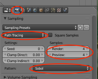
The most intuitive and most straight forward settings to influence antialiasing sampling and render speed can be found on the Render panel, Sampling section. By default, the settings are as follows:

The option "Method to sample light and material" is by default set to "Path Tracing". If you want to tweak you render quality in detail, put it to "Branched Path Tracing" which gives you access to every knob and button to influence individually the sampling method for any shader type used in the scene:

Aditionally, only with the sampling method set to "Branched", the option to influence the number of samples of a light source becomes available (see above).

Speed versus Output Quality Comparison

So - knowing all these settings above, I asked myself how do these influence the quality and rendering speed? To check this I created a very simple scene with a cube (diffuse BSD) on a plane (Mix shader Glossy BSD + Diffuse BSD) and one Area Light, the hardware I used was my MacBook Pro at home. The output dimension was 50% of 1920x1024 (i.e. 960x512 pixel)

Baseline: minimum quality maximum speed

• Sampling Method: "Path Tracing"
• Render Samples: 1
• Render Layers Samples: 0
• -> Render Time 1.85 s

Increasing Samples on Render panel

4 samples / 4.4 s: 

8 samples / 7.7 s:

For this image dimension the image quality does not increase significantly if one increases the number of samples. Hence here only the render times:

16 samples / 14.4 s

32 samples / 27 s

Increasing Samples on Render Layer panel

The render time / quality behavior behaves exactly the same as the Samples on the Render panel with "Path Tracing" active on the Render panel

Same for Branched Path Tracing

Baseline all Samples to "1", "0" on Render Layers

render time = 2.2 s

Influence of Samples on Render Layers, all other at "1"

4 samples / 5.8 s

8 samples / 10.6 s

16 samples / 20.2 s

32 samples / 39.3 s

Influence of Samples on Light -> Data

Samples on Render panel = "1", Samples on Render Layer panel = "4"

1 light sample / 5.8 s

4 light samples / 9.2 s

8 light samples / 13.2 s

16 light samples / 21.5 s

32 light samples / 38.3 s

The influence of the light samples are mostly visible if you are dealing with diffuse reflections / bright spots on surfaces. The effect can be seen if you focus your attention on the bright spot on the lower edge of the image compared to those above:

Influence of AA Samples on Render panel

Render Layers samples = "0", Light -> Data samples = 1, Shader samples on Render panel = 1

4 AA samples / 5.9 s

8 AA samples / 10.7 s

16 AA samples / 20.3 s

32 AA samples / 39.5 s

The results are comparable with those of "standard" Path Branching. Specular reflections / highlights remain grainy/noisy even at high sampling rates.

Influence of "Diffuse" Shader Samples

Render Layers samples = "0", Light -> Data samples = 4, AA samples on Render panel = 4

All other shader samples set to 1

1 Diffuse shader sample / 9.1 s

4 Diffuse shader samples / 12,2 s

8 Diffuse shader samples / 16.5 s

16 Diffuse shader samples / 25.4 s

32 Diffuse shader samples / 41.7 s

Increasing the other shader's samples increases the render time by a similar amount - e.g. setting the samples for the glossy shader up to 32 adds another 40 seconds to the total render time. The Light -> Data -> Samples impacts the rendering time not as an adding but multiplying factor. E.g. if the light samples are increased by a factor of 8, rendering time increases by this factor as well.